MARS Rover GNC

With my GNC implemented and well tested, I then proved it to Silver and added Gold properties, which I also proved. Throughout, I used agentic AI to accelerate my work.

The results? Silver was proved automatically and autonomously by the agent. Gold contracts were written automatically and autonomously by the agent. The Gold proofs were a mixed result (a useful failure, if you will) but the details matter, so read on!

If you’re eager to grab the code, you can find it here on the mars-rover-gnc branch.

Simulator Enhancement

Disturbances

The initial state of the simulator had the Rover moving around on a perfectly flat plane that offered perfect traction. This mirrored the state of the setup we’d have at trade shows, where the Rover moved around on a flat picture of the Martian surface.

But a flat surface is boring for GNC: there’s not much control that’s needed, and state estimation becomes trivial. So I added a disturbance model to the simulator. Now, when the simulator starts up, it generates a random height map. Using the height map, the simulator computes per-wheel slippage. The Rover can no longer travel in a straight line without positive control.

MARS Rover Sensors

I added three kinds of sensors to the Rover in the simulator:

wheel encoders
GPS
MEMS gyroscope

The wheel encoders are 48-tooth incremental encoders that reset when polled. They accumulate a count of encoder teeth into a 16-bit signed integer (so we can detect forward and reverse rotation). At a top speed of about 80 rpm, this gives about 8.5 minutes of accumulation before the counter rolls over, which seems generous but plausible. Only the four corner wheels have encoders; the middle wheels are ignored. The SPARK code polls the encoders roughly every 40 ms.

GPS doesn’t exist on Mars, of course, but for the purpose of this exercise, I chose to imagine that it does. GPS is modeled as gaussian noise added to the true X,Y position of the Rover. Sigma is a bit larger than the Rover body width (10 cm sigma v 7.7 cm width), resulting in GPS measurements that are visibly offset for the Rover’s true location. GPS updates at 2Hz.

SPARK fuses the information from the encoders, GPS, and gyro using an extended Kalman filter (EKF, explained in more detail in the next section). In the absence of disturbances, the filter’s performance was acceptable. With disturbances, however, the filter diverged from truth very quickly because there was no meaningful way to cancel heading drift except through successive GPS readings, and the rate at which GPS updated was far too slow for this purpose.

So I added a third sensor: a MEMS gyroscope that reports dTheta, the angular rate of the vehicle body around the Z axis, directly. The gyro outputs a signed 16-bit integer and offers a range of ±4.0 rad/s and a resolution of 0.000122 rad/s (0.007 deg/s).

Once added to the EKF, these sensors are adequate to allow SPARK to derive an acceptably accurate estimate of the Rover’s heading and position, even in the presence of disturbances. This estimation is the basis of GNC.

Waypoints

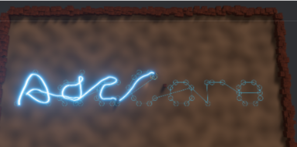
GNC needs something to track. The simplest solution is to give the Rover a list of waypoints and ask it to navigate from one to the next. Rather than building these from a file or interactively in the simulator, I added a text-to-waypoint capability. When I launch the simulator, I can provide a string; this is then converted into a list of waypoints that, when followed by the Rover, will trace the letters in the string.

Visualization Enhancements

The purpose of the simulator is not only to feed data into the SPARK via the hardware abstraction layer (HAL), but also to show you what the Rover is doing. So I added visualizations of SPARK’s state estimate, the waypoints and the path that interpolates them, and a glowing trail behind the Rover so you can see where it’s been.

SPARK Enhancement

Hardware Abstraction Layer

Straightforward additions to the HAL give SPARK the ability to poll the new sensor values through defined interfaces.

The HAL also now provides interfaces that SPARK can use to advertise its state. These might feel like a bit of a stretch (why would the Rover hardware need these interfaces?) but the Rover hardware already provided a status display, so I think it’s a defensible addition. We could imagine that the Rover hardware has nonvolatile storage to log state (i.e., a flight data recorder). For now, these interfaces allow us to visualize the Rover’s state estimate in the simulator and, as importantly, implement data logging for analysis and faster-than-real-time replay testing of the GNC.

Estimator

The estimator provides the critical information that GNC uses for loop closure: where is the Rover and what is its heading?

The sensors that I added to the simulator were chosen to be reasonably realistic, to offer sufficient information for good (even excellent) state estimation, and not to be sufficient on their own. The role of the estimator is to fuse the input from all of the sensors into a single position + heading solution that is then fed into GNC.

A standard approach for combining noisy, heterogeneous sensor measurements into a single best-estimate of system state is to use an extended Kalman filter. It works in two alternating steps: a predict step, which advances the state estimate forward in time using a model of the system’s dynamics (the Rover’s kinematics, in our case), and an update step, which corrects that estimate whenever a measurement arrives. The "extended" part means the filter handles nonlinear dynamics (as Rover kinematics are) by linearizing around the current estimate at each step.

The filter's state vector has four components: X position, Y position, heading θ, and an odometry scale factor. The first three are the obvious ones. The fourth is less obvious but important: it represents the ratio of actual ground displacement to encoder-implied displacement — in other words, how much the wheels are slipping. Rather than assuming perfect traction, the filter treats wheel-ground coupling as uncertain and estimates the scale factor continuously, bounding it to the range [0.1, 2.0] to prevent divergence: over time, the filter learns how slippery the ground is overall. Without this term, the filter would continuously overestimate the forward velocity of the Rover, so that the Rover’s true location always lagged behind the estimated location.

The predict step runs every 40 ms and advances X, Y, and θ using encoder odometry and gyro integration. The scale factor uses a random-walk model — its predicted mean is held constant each cycle, but its uncertainty grows, allowing GPS corrections in the update step to refine it. The update step runs only when a fresh GPS fix arrives (2 Hz). GPS touches only the X and Y components of the state; heading is left to the gyro.

One tuning detail worth noting: the filter's assumed GPS measurement noise (R_GPS = 0.09 m², implying σ = 0.3 m) is set three times as large as the actual simulated noise (σ = 0.1 m). This is deliberate — it makes the filter conservative about snapping to GPS fixes. The result is a smoother position estimate at the cost of slower convergence when there is a major disturbance to the Rover’s position or when the filter is (re)initialized.

Guidance

Our guidance loop is simple. When we’re not tracking a waypoint, we pull the first waypoint from the list. When we are tracking a waypoint, we ask if we’ve reached it (to within an appropriate tolerance). When we’re out of waypoints to track, we exit GNC mode and return to the Rover’s previous autonomous/remote-control loop.

Guidance waits until the estimator is fully initialized (after the first GPS fix arrives) before engaging. So the Rover is still for half a second on simulation startup.

Navigation + Control

For the current demo, navigation and control are unified into a pure-pursuit path-following algorithm. At every step, the Rover steers towards the current waypoint. The steering angle is proportional to the heading error, clamped to ±40 degrees. Moreover, the Rover uses its 4-wheel independent steering here: the front wheels steer in the error direction while the rear wheels counter-steer by the same angle. This coordinated 4WIS gives a tighter turn radius than front-steer alone.

This means that, as disturbances from the terrain push the Rover off course, it steers back towards the current waypoint - but not back towards the line it was previously tracking (that would be cross-track correction, which would be proper control). Pure-pursuit is simple and effective. The resulting ground track is endearingly wobbly.

One modification we did make to pure-pursuit was to engage the Rover’s zero-radius turn (4WID) mode whenever the angular difference between the current heading and desired heading (to point back to the waypoint) exceeds 45 degrees. This allows the Rover to make very sharp heading adjustments, which is important when tracing many letters!

Not forgetting our safety requirement, obstacle avoidance remains active throughout path following. If sonar detects something within Safety_Distance, power is zeroed regardless of what the path-following algorithm wants and the Rover simply halts. And waits for someone to move the obstacle out of its path. Obstacle circumnavigation would be an interesting possible future enhancement to the demo!

Refactoring: Not a Sidequest

Refactoring is important for any code and is good software-engineering practice. But it’s especially important for proof. SPARK is modular, but large subprograms may still pose problems for SPARK’s provers: they tend to start drowning in proof context and thus stop finding proofs in a timely fashion (or at all).

There were two steps that I undertook to get ready for proof: DRYing up the code and tightening the bounds on the numeric types.

DRYing the Code

Initially, the agent wrote the body of the GNC package twice: once in the demo’s device directory and again in the demo’s binding directory. This code duplication was not only concerning but also pointed to an underlying issue with abstraction.

Agents - even more so than people - do best when they’re given really solid tools for automatic verification and validation (this is why SPARK + AI is such a successful pairing!). So before the agent and I dove in to work on refactoring, we built a faster-than-real-time testing framework based on replaying previously recorded log files. The workflow is:

Run the simulation, logging data from the simulator and the GNC. This is real-time and interactive, insofar as the user may have to remove obstacles and decide when to stop simulating and thus recording data.
Run a specialized harness that feeds logged data back into the GNC and compares GNC outputs - estimates and actuator commands - against the log. This is faster-than-real-time (almost instantaneous) and requires no user involvement. The result is a list of pass/fail for each row of logged data and a final summary at the end of the run.

The log contains 24 columns including both ground truth (from the physics simulation) and SPARK’s EKF estimate, so divergence between the two is also visible in replay — not just actuator output mismatches. Waypoints are saved alongside each log in a sidecar file, ensuring the replay runs the exact same path as the original.

Running a time-sensitive system like an EKF from logged data is tricky. Ada's Delay_Milliseconds(40) call, instead of sleeping, becomes a two-phase synchronization barrier: Ada signals the harness that a cycle is complete, the harness reads Ada's now-stable outputs and compares them, injects the next sensor window, then releases Ada to continue. Ada never knows it's running in replay mode; it calls the same mars_rover_clock() function it always does, but gets virtual time instead of wall time. This is why "close enough" is as good as it gets. Any floating-point non-determinism between runs accumulates, but the barrier ensures the comparison always happens at the right moment. Although after several iterations the results don’t quite line up perfectly, they’re close enough to build very strong confidence that, were a refactor to change the EKF or GNC behavior at all, the log would quickly diverge into all failures.

Armed with this tool, the agent successfully performed my refactoring tasks, and I didn’t have to worry that we’d broken anything!

Tightening the Numeric Bounds

A quick glance at the Rover.Estimation code revealed that the agent, while using good numeric subtypes for the HAL, used generic Floats everywhere for the implementation of the estimator state and the Kalman filter Predict and Update methods. But raw Integer and Float types are the enemy of proving absence of overflow, see also this blog post for more context..

The gnatprove skill that is included in AdaCore’s open-sourced skills repository has instructions that encourage the agent to use numeric subtypes, but the agent’s ability to follow this instruction while in the midst of a proof campaign is hit or miss.

So I asked the agent to go through all of the raw Float and Integer types up front and, using domain knowledge from the simulator, refactor these to use numeric subtypes. For each numeric subtype, I asked the agent to use constants for the min and max values and to document clearly how those constants related to values in the simulation and when they need to be revisited: these constants represent assumptions about the interface between the SPARK code and the physical world; they thus require careful validation. In a typical embedded, high-integrity system, this information would be provided in the form of an Interface Control Document (ICD) or similar.

The result of the agent’s work is tight numeric types for most instances of Integer and Float; these made moving on to proof possible.

SPARK Proof

`Rover.Estimation` - Silver

Invoking the gnatprove skill, I asked the agent to prove Rover.Estimation to SPARK silver - absence of runtime errors.

Following the workflow, the agent ran an initial run with gnatprove. Then, it asked me an insightful question: if it could revert the numeric subtype for the X and Y elements of Rover.Estimation.State to pure Float. Its rationale: Update would definitely push the state elements outside of their numeric subtype due to the range of possible values from the GPS, given GPS noise.

This was believable - but missed the core of the problem. For any closed-loop computation like an EKF, SPARK must prove not only that, given the constraints on the computation’s inputs (including state), the body is free from runtime errors like overflow, but also that the computation’s outputs (including state update) lie within the constraints on the inputs (including state). Said differently, the proof must show that the computation is closed under the types used to describe its state. This is essentially induction: given EKF state + inputs at step N, show that EKF state at step N+1 satisfies its constraints.

Shifting to pure Float, I pointed out to the agent, wouldn’t solve the problem. It just moves it to more extreme cases.

After quite a long time “thinking” about my response, the agent proposed a refactoring of the EKF that would allow it to establish the needed properties piecewise. It made this refactoring, showed that the refactoring didn’t cause regressions in the replay test, and started on the proof.

The proof took about four hours to reach a state that appeared to be complete. The agent returned a state in which Rover.Estimation proved cleanly at level=2. This meant that none of the intermediate computations in the EKF could ever exceed their bounds - a significant accomplishment, given the filter is a mess of nonlinear, floating-point arithmetic.

The approach taken by the agent was to introduce about 10 lemmas whose purpose was to isolate the proof that an operation (generally nonlinear) would fall within the bounds of a given numeric subtype. Each of these lemmas had a null body; the win occurs because the computation + bounds check was isolated from the context of the overall filter Predict subprogram, allowing the provers to find a proof of the lemma automatically; within the context of the subprogram, the provers were not able to find a proof at level=2. (This is, alas, a common challenge with SPARK proofs.) Aside from the frequent invocation of the lemmas, the annotation burden in the subprogram was overall not very high.

The agent made the decision to limit the preconditions on Predict and Update to large-but-sensible values of State and Covariance and prove absence of runtime errors from there. The result means that, provided Predict and Update are always called within these limits, none of the computations will overflow. The agent set types of State and Covariance to Float during this process (contrary to the outcome of our discussion).

Initially, I was irritated that the agent set State and Covariance to Float. But as I dug into the problem in conversation with the agent, I realized that, since I asked for a silver proof of the Rover.Estimation, this was actually an acceptable outcome. The agent had done what I asked / met my highest-level requirement: raise the Rover.Estimator code to SPARK silver.

But then I decided I really wanted a gold-level proof.

`Rover.Estimation` - Gold

The estimator is called by GNC in a loop. Predict is called continuously, in a loop. Periodically, when a GPS fix arrives, Update is called; this happens every 13 iterations (GPS updates at 2Hz and the fundamental frame rate is 25Hz).

Because Rover.Estimator now has preconditions on Predict and Update (from the silver proof), GNC will need to show that the result of Predict and Update on state S and covariance P is always such that Predict or Update can be called again, on the next loop. So Predict must have a postcondition sufficient to guarantee that Predict or Update can be called in the next iteration; Update must have a postcondition sufficient to guarantee that Predict can be called in the next iteration. Otherwise, GNC’s own silver proof cannot succeed, since meeting a called-subprogram’s precondition is part of showing Absence of Runtime Errors.

The intuitively easy way to do this is to ensure that the postcondition on Predict includes its own and Update’s precondition. Likewise to ensure that the postcondition on Update includes the precondition on Predict. Then, we’re assured that we can call Predict as many times in a row as we like and that we can call Update whenever we want; all we have to do is capture the postcondition in a loop invariant and SPARK will prove that the precondition is always satisfied.

Unfortunately, the math doesn’t work out. Indeed, the entire concept is flawed. If we had this property in Predict, we wouldn’t need Update: we’d magically know that our estimator’s predictions always remain bounded in whatever region we defined, absent any correction. But there’s nothing given to the estimator that tells it the Rover can’t drive forever in a given direction. And in the presence of disturbances, errors accumulate and need correction. That’s part of the point of the estimator.

What we might do is say that, if we start with S and P sufficiently well inside the precondition bounds on each, the changes made by each call to Predict are small enough that even after calling Predict 12 times in a row, we’re still guaranteed to satisfy its precondition on the 13th call. And then we can say that Update will move the values of S and P back into that region, so that we can make 13 calls to Predict again. The call sequence looks like this:

Init → (Predict¹³ → Update)*

This region is analogous to the inductive invariant that I mentioned in a footnote on the first Mars Rover post; the precondition is then analogous to the safety invariant. Update must establish a strictly stronger property than is needed for one call to Predict so that we can be sure we can call Predict 13 times in a row, safely.

These, then, are our gold-level properties:

Init establishes the inductive invariant for our base case (which is trivial).
Update establishes the inductive invariant provided we’re within our safety region
Predict establishes the rate of departure from the inductive invariant, if you will, so that we can show that doing that 13 times is okay

Unfortunately, this is terribly hard to do in the floating-point domain. While the math for these properties works out in the real domain, it typically doesn’t in the floating-point domain. Interacting heavily with the agent, I pursued several approaches; ultimately, I was forced to abandon each of them. Either the property was falsifiable (e.g., I refuted a critical lemma to one approach using GNATfuzz) or the provable bounds grew too quickly within one step to enable proof over multiple steps.

Arguably, this entire problem is a bit of a bad fit for SPARK. I’ve said before that SPARK should not be used to prove properties of closed-loop dynamical systems, especially not control-theoretic properties. An extended Kalman filter is at least right on the line if not across it: there are perfectly applicable tools from linear algebra, controls, and real analysis that will establish the properties of a Kalman filter. I could have (and perhaps should have) used those: done a pen-and-paper proof and, through careful review, linked my proof to the implementation of my estimator.

But I really wanted to show that SPARK is capable of proving a property like this (even if it’s probably not worth it). And I wanted to show that an AI agent could drive SPARK to the proof. And working on all this allowed me to make many important refinements to AdaCore’s gnatprove Skill, which you can use with your agent of choice in your own work with SPARK.

So while I didn’t accomplish my objective, I did validate that agentic AI is:

able to derive and formalize extremely complex gold-level properties
operates as a strong partner for domain-heavy, gold-level proofs.

`Rover.Estimation` - Weaker Gold

I intended to fall back to my working Silver proof and continue from there. But I misread my git log and accidentally rolled back to an early Gold state: insufficient, but still interesting postconditions on Predict and Update. I ran the proof, found a few errors, and asked the agent to fix them and apply my lemma refactoring discipline. It did so, leaving only two postconditions unproved - these depended on a property I’d already established cannot be proved!

So I instructed the agent to protect these postconditions (which we believe to be true and just cannot currently prove) with a runtime check, raising a user-defined exception that is handled at the GNC level.

These contracts don’t establish the Init → (Predict¹³ → Update)* chain that I wanted, so I dealt with that concern using runtime checks in the GNC.

GNC - Silver

After the failure to prove a satisfactory Gold property on Rover.Estimator, proving GNC to Silver was refreshingly easy. The agent accomplished this in nearly one shot. It introduced an indefensible clamp on the gyro’s Integer to Float subtype scaling. When I challenged it on this, it removed the clamp, refactored the conversion into an expression function, and the subtype proved cleanly.

Of course, there are residual runtime checks in GNC, as I said above. At each step, the precondition on Predict and, when it’s time to call, Update is checked. If the precondition would fail, an exception is raised. Ultimately, this exception is handled in Rover.Tasks, and shuts down GNC, reverting to the (Autonomous → Remote Control)* loop that was there from before.

Importantly, SPARK tells us that with these exceptions (pun intended), no other runtime errors are possible. We know precisely what may go wrong at runtime and how it will be handled.

Conclusion

Agentic AI has come a long way in the past year. A year ago, practically nobody was talking about agentic AI; now, it’s ubiquitous!

Large language models are able to generate good SPARK code. On top of that, with our gnatprove skill, the agent is able to lift the SPARK code and prove it to Silver automatically and autonomously - even complex, Float-heavy code like the Rover.Estimator! The agent is able to write strong, Gold contracts. Yes, proving strong Gold contracts is not a slam dunk, but, as I admitted above, this wasn’t the best fit for SPARK.

But my message is: while there’s obvious room for improvement, you should be using SPARK + AI now in your high-integrity software projects. The wins are real.

We’ve said for years that you simply can’t write better code than with SPARK. Now I’m saying that you simply can’t generate better code with agentic AI than with SPARK. It’s worth the extra tokens to get the code right, and SPARK + AI can get you across that finish line.

Where do we go from here? I encourage you to clone the repo here, switch to the mars-rover-gnc branch, and try things out for yourself. All tools are available in open source and can be installed through Alire. If you’re a professional developer of high-integrity software and want to hear more about how SPARK Pro can help you, reach out to our sales team; we’d be delighted to discuss your needs and our solutions. And keep an eye on our blog: we have more AI-related content in the pipe that we’re excited to share!

¹One reason this approach may be preferred is that, for SPARK to prove these properties, the parameters that could be used to tune the extended Kalman filter are constants. But tuning parameters like these are often left “unlocked” in code and modified via configuration files during integration and system testing. A more general proof of convergence for the filter would better support this kind of workflow, but would likely be unapproachable for SPARK.